39 conditional formatting pivot table row labels

Overwrite pivot table conditional format based on row label As far as I know, using the one rule in the Conditional formatting, we can only format the cells with one color if the condition is true and if the same condition is false, the formatting of the cell will be blank and if both conditions are true, the formatting of cell depends on the highest ranking/priority of the rules in Conditional formatting. Conditional Formatting in Pivot Table (Example) | How To Apply? - EDUCBA Click on any cell in the pivot table > Go to the HOME tab > Click on Conditional Formatting option under Styles option > Click on Manage Rules option. It will open a Rules Manager dialog box. Click on the Edit Rule tab, as shown in the below screenshot. It will open the Editing Rule formatting window. Refer to the below screenshot.

How to Use Pivot Table Field Settings and Value Field Setting - Excel Tip How to Refresh Pivot Charts | To refresh a pivot table we have a simple button of refresh pivot table in the ribbon. Or you can right click on the pivot table. Here's how you do it. Conditional Formatting for Pivot Table | Conditional formatting in pivot tables is the same as the conditional formatting on normal data. But you need to be careful ...

Conditional formatting pivot table row labels

Progress Doughnut Chart with Conditional Formatting in Excel Mar 24, 2017 · Step 3 – Apply the Formatting & Data Labels. Finally, we need to clean up the formatting. This is the same basic process as step 3 above. The only difference is that we create three separate text boxes, one for each level. This allows us to change the color of each textbox to match the bar color. Conditional Format Pivot Table Row - Chandoo.org Select the entire row, and when you apply the conditional format, make the column reference absolute. So, say we want the entire row 2 to be formatted if cell in col B = 5. formula would be: =$B2=5 Design the layout and format of a PivotTable To change the format of the PivotTable, you can apply a predefined style, banded rows, and conditional formatting. Windows Web Mac Changing the layout form of a PivotTable Change a PivotTable to compact, outline, or tabular form Change the way item labels are displayed in a layout form Change the field arrangement in a PivotTable

Conditional formatting pivot table row labels. Pivot Table Conditional Formatting with VBA - Peltier Tech A reader encountered problems applying conditional formatting to a pivot table. I tried it myself, using the same kind of formulas I would have applied in a regular worksheet range, and had no problem. ... including what I think you meant with your last suggestions (and Text1 is one of my Row Labels, and Text is one of the names populating ... Conditional Formatting in Pivot Table - WallStreetMojo We must follow the steps to apply conditional formatting in the pivot table. First, we must select the data. Then, in the "Insert" Tab, click on "Pivot Tables." As a result, a dialog box appears. Next, we must insert the pivot table in a new worksheet by clicking "OK." Currently, a pivot table is blank. Next, we need to bring in the values. Pivot Table Conditional Formatting Based on Another Column ... - ExcelDemy We can conditionally format the entire Pivot Table depending on the blanks. Step 1: Repeat Step 1 of Method 1 then the New Formatting Rule window will open. Here in the New Formatting Rule window, Select the 3rd and 2nd options from Apply Rule to and Select a Rule Type command box respectively. Inside Edit the Rule Description dialog box, Conditional Formatting on Pivot Table row labels Re: Conditional Formatting on Pivot Table row labels Hi Dilip, The date is a "date" and not a text. What I mean is each cell in A should be compared with the 3 dates in E and should do the conditional formatting (excel icon sets) accordingly. If you see the cell A in srcFromWorkSheet you know what I mean. Please let me know if you have any queries.

How to Create a Pivot Table in Power BI - Goodly Oct 19, 2018 · To create a Pivot, pick up the “Matrix Visual” and NOT the Table visual. As soon as you create a Matrix, you’ll get similar options like you do in Excel i.e. Rows, Columns and Values. You’ll also find that the Matrix looks a lot cleaner than a Pivot in Excel. Next, lets move on to some formatting features of the Pivot Table . 2 ... Pivot table conditional formatting based on row label Kerja, Pekerjaan ... Cari pekerjaan yang berkaitan dengan Pivot table conditional formatting based on row label atau upah di pasaran bebas terbesar di dunia dengan pekerjaan 21 m +. Ia percuma untuk mendaftar dan bida pada pekerjaan. Formatting tables and pivot tables in Amazon QuickSight To add a label for totals and subtotals. In the Format visual pane, choose Total or Subtotal. For Label, enter a word or short phrase. In pivot tables, you can also add labels to column totals and subtotals. To do so, enter a word or short phrase for Label in the Columns section. To format totals and subtotals text. What Are Columns and Rows? - Lifewire May 28, 2020 · Selecting a whole row is similar: click the row number or use Shift+Spacebar. To move through a worksheet, click cells or use the scroll bars on the screen, but when dealing with larger worksheets, it's often easier to use the keyboard. ... Use Excel's Power to Print Labels in No Time. Spreadsheet Cells: What They Are and How They're Used. How ...

Pivot Table Grouping, Ungrouping And Conditional Formatting So let's drag the Age under the Rows area to create our Pivot table. #1) Right-click on any number in the pivot table. #2) On the context menu, click Group. #3) Grouping dialog box appears, in this example, the least number is 25, so by default the Starting number is entered as 25, and you can change if necessary. Re-Apply Pivot Table Conditional Formatting - yoursumbuddy In cases where the conditional formatting might not apply to the leftmost row label, I've still applied it to that column, but modified the condition to check which column it's in. This function can be modified and called from a SheetPivotTableUpdate event, so when users or code updates a pivot table it re-applies automatically. Microsoft Excel Manual - Administration and Finance Column Labels – Adds columns to the table based on fields in that area; Row Labels – Adds rows to the table based on fields in that area; Values – Performs an Auto Sum action in the table based on the fields in that area. In a pivot table, you can sort and filter like you can with any other data range. To Change the Summary Calculation ... Pivot Table: Pivot table conditional formatting | Exceljet Select any cell in the data you wish to format and then choose "New rule" from the conditional formatting menu on the Home tab of the ribbon. At the top of the window, you will see setting for which cells to apply conditional formatting to. For the example shown, we want: "All cells showing sum of "sales values" for name and "date"

How to use conditional formatting in decorating pivot tables | Basic Excel Tutorial

Pivot Chart Formatting Changes When Filtered - Peltier Tech Apr 07, 2014 · Here is Jon A’s original unfiltered pivot table on the left and mine (Jon P’s) on the right. His has six columns of values, mine has two. There are several pivot charts below each pivot table. The first chart under each pivot table has only default formatting applied: blue for series 1, orange for series two, gray for series three, etc.

Formatting Tips for Pivot Tables - Goodly

Pivot table conditional formatting based on column value jobs Search for jobs related to Pivot table conditional formatting based on column value or hire on the world's largest freelancing marketplace with 21m+ jobs. It's free to sign up and bid on jobs.

How To Remove Blank In Pivot Table | Decoration Ideas For Thanksgiving

Issue with conditional formatting in pivot table | General Excel ... No, you either have totals on or off for all columns. You could use some conditional formatting to hide the totals by formatting the font in the same colour as the total cell. You'd need to use regular conditional formatting for this, i.e. not PivotTable conditional formatting. Apply it to the column, where the row label contains 'Total'.

How To Find And Remove Duplicates In A Pivot Table - MS Excel | Excel In Excel

How to Group Numbers in Pivot Table in Excel - Trump Excel Select any cells in the row labels that have the sales value. Go to Analyze –> Group –> Group Selection. In the grouping dialog box, specify the Starting at, Ending at, and By values. ... How to Apply Conditional Formatting in a Pivot Table in Excel. How to Add and Use an Excel Pivot Table Calculated Field. How to Replace Blank Cells with ...

How to Apply Data Bars in Pivot Table - MS Excel | Excel In Excel

Format Pivot Table Labels Based on Date Range In the pivot table, remove any filters that have been applied - all the rows need to be visible before you apply the conditional formatting. Select all the dates in the Row Labels that you want to format. On the Ribbon, click the Home tab, and then in the Styles group, click Conditional Formatting.

Pivot Table Conditional Formatting with VBA - Peltier Tech Blog

Excel VBA: Conditional Format of Pivot Table based on Column Label ... myPivotSourceName = myPivotField.Name. Then rather than referencing the data field with the pivot field object, I referenced the DataRange with the string: myPivotTable.PivotFields (myPivotSourceName).DataRange.Select. Works perfectly and is completely portable for any pivottable on any sheet with any fields. excel vba.

How to use conditional formatting in decorating pivot tables – Basic Excel Tutorial

How to Replace Blank Cells with Zeros in Excel Pivot Tables Excel Pivot Tables has an option to quickly replace blank cells with zeroes. Here is how to do this: Right-click any cell in the Pivot Table and select Pivot Table Options. In Pivot Table Options Dialogue Box, within the Layout & Format tab, make sure that the For Empty cells show option is checked, and enter 0 in the field next to it.

microsoft office - Excel 2013 table formatting - Super User

Conditional Formatting Using Custom Measure - Power BI Sep 28, 2020 · Let us consider the following table visual: I have got sales by clothing category, by day of a week in the above table visual. Now, my task is to give a custom conditional formatting to the Day of Week column above based on the Clothing Category. For example - Clothing Category = Jackets should be GREEN. Clothing Category = Jeans should be BLUE

How to Sort Pivot Table Row Labels, Column Field Labels and Data Values with Excel VBA Macro ...

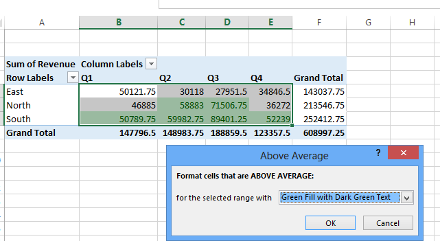
How to Apply Conditional Formatting to Pivot Tables So in this post I explain how to apply conditional formatting for pivot tables. 1. Select a cell in the Values area The first step is to select a cell in the Values area of the pivot table. If your pivot table has multiple fields in the Values area, select a cell for the field you want to apply the formatting to. 2. Apply Conditional Formatting

How to Apply Conditional Formatting to a Pivot Table + [5 Examples]

How to remove bold font of pivot table in Excel? - ExtendOffice The normal Bold feature can’t help us to un-bold the row labels in pivot table, but we can apply the powerful function – Conditional Formatting to solve this problem. Please do as follows: 1. Select the bold font row you want to un-bold in the pivot table, or you can press Ctrl key to select multiple bold font rows as your need. See screenshot:

How to Sort Pivot Table Row Labels, Column Field Labels and Data Values with Excel VBA Macro ...

Design the layout and format of a PivotTable To change the format of the PivotTable, you can apply a predefined style, banded rows, and conditional formatting. Windows Web Mac Changing the layout form of a PivotTable Change a PivotTable to compact, outline, or tabular form Change the way item labels are displayed in a layout form Change the field arrangement in a PivotTable

Conditional Formatting in Pivot Table (Example) | How To Apply?

Conditional Format Pivot Table Row - Chandoo.org Select the entire row, and when you apply the conditional format, make the column reference absolute. So, say we want the entire row 2 to be formatted if cell in col B = 5. formula would be: =$B2=5