44 excel pie chart add labels
Microsoft Excel Tutorials: Add Data Labels to a Pie Chart The chart is selected when you can see all those blue circles surrounding it. Now right click the chart. You should get the following menu: From the menu, select Add Data Labels. New data labels will then appear on your chart: The values are in percentages in Excel 2007, however. To change this, right click your chart again. c# - Add data labels to excel pie chart - Stack Overflow Add data labels to excel pie chart. Ask Question Asked 9 years, 9 months ago. Modified 5 years, 10 months ago. Viewed 9k times 4 1. I am drawing a pie chart with some data: private void DrawFractionChart(Excel.Worksheet activeSheet, Excel.ChartObjects xlCharts, Excel.Range xRange, Excel.Range yRange) { Excel.ChartObject myChart = (Excel ...
Multiple data labels (in separate locations on chart) You can do it in a single chart. Create the chart so it has 2 columns of data. At first only the 1 column of data will be displayed. Move that series to the secondary axis. You can now apply different data labels to each series. Attached Files 819208.xlsx (13.8 KB, 263 views) Download Cheers Andy Register To Reply

Excel pie chart add labels
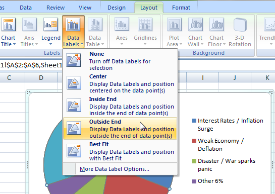
How To Add Axis Labels In Excel [Step-By-Step Tutorial] First off, you have to click the chart and click the plus (+) icon on the upper-right side. Then, check the tickbox for 'Axis Titles'. If you would only like to add a title/label for one axis (horizontal or vertical), click the right arrow beside 'Axis Titles' and select which axis you would like to add a title/label. Add data labels and callouts to charts in Excel 365 ... The steps that I will share in this guide apply to Excel 2021 / 2019 / 2016. Step #1: After generating the chart in Excel, right-click anywhere within the chart and select Add labels . Note that you can also select the very handy option of Adding data Callouts. How to Create Pie Charts in Excel (In Easy Steps) 6. Create the pie chart (repeat steps 2-3). 7. Click the legend at the bottom and press Delete. 8. Select the pie chart. 9. Click the + button on the right side of the chart and click the check box next to Data Labels. 10. Click the paintbrush icon on the right side of the chart and change the color scheme of the pie chart. Result: 11.
Excel pie chart add labels. How to Create and Format a Pie Chart in Excel - Lifewire Select the plot area of the pie chart. Right-click the chart. Select Add Data Labels . Select Add Data Labels. In this example, the sales for each cookie is added to the slices of the pie chart. Change Colors When a chart is created in Excel, or whenever an existing chart is selected, two additional tabs are added to the ribbon. Excel 2010 pie chart data labels in case of "Best Fit" Based on my tested in Excel 2010, the data labels in the "Inside" or "Outside" is based on the data source. If the gap between the data is big, the data labels and leader lines is "outside" the chart. And if the gap between the data is small, the data labels and leader lines is "inside" the chart. Regards, George Zhao TechNet Community Support Add a DATA LABEL to ONE POINT on a chart in Excel | Excel ... Method — add one data label to a chart line Steps shown in the video above:. Click on the chart line to add the data point to. All the data points will be highlighted.; Click again on the single point that you want to add a data label to.; Right-click and select 'Add data label' This is the key step! Excel custom pie chart labels - Microsoft Community Excel custom pie chart labels. I want to use a pivot table to make a pie chart out of this. I want each of the pieces of the pie to contain the number of entries and between parentheses the percentage. So in the "Yes" piece, there should be '3 (33%)'. Actually, if I hover the pie chart in Excel, I get exactly the notation O want!
Inserting Data Label in the Color Legend of a pie chart ... Re: Inserting Data Label in the Color Legend of a pie chart @SabrinaFr There is no built-in way to do that, but you can use a trick: see Add Percent Values in Pie Chart Legend (Excel 2010) Pie Chart in Excel - Inserting, Formatting, Filtering ... To add Data Labels, Click on the + icon on the top right corner of the chart and mark the data label checkbox. You can also unmark the legends as we will add legend keys in the data labels. We can also format these data labels to show both percentage contribution and legend:- Right click on the Data Labels on the chart. Pie Chart in Excel | How to Create Pie Chart | Step-by ... Follow the below steps to create your first PIE CHART in Excel. Step 1: Do not select the data; rather, place a cursor outside the data and insert one PIE CHART. Go to the Insert tab and click on a PIE. Step 2: once you click on a 2-D Pie chart, it will insert the blank chart as shown in the below image. Adding data labels to a pie chart - Excel General - OzGrid ... Re: Adding data labels to a pie chart. Thanks again, norie. Really appreciate the help. I tried recording a macro while doing it manually (before my first post). But it didn't record anything about labels, much less making them bold.
Creating Pie Chart and Adding/Formatting Data Labels (Excel) Creating Pie Chart and Adding/Formatting Data Labels (Excel) Add or remove data labels in a chart - support.microsoft.com Click the data series or chart. To label one data point, after clicking the series, click that data point. In the upper right corner, next to the chart, click Add Chart Element > Data Labels. To change the location, click the arrow, and choose an option. If you want to show your data label inside a text bubble shape, click Data Callout. Add / Move Data Labels in Charts - Excel & Google Sheets ... Adding and Moving Data Labels in Google Sheets Starting with your Data. We'll start with the same dataset that we went over in Excel to review how to add and move data labels to charts. Add and Move Data Labels in Google Sheets. Double Click Chart; Select Customize under Chart Editor; Select Series . 4. Check Data Labels. 5. Edit titles or data labels in a chart On a chart, click the label that you want to link to a corresponding worksheet cell. On the worksheet, click in the formula bar, and then type an equal sign (=). Select the worksheet cell that contains the data or text that you want to display in your chart. You can also type the reference to the worksheet cell in the formula bar.

| Pryor Learning Solutions
excel - Positioning data labels in pie chart - Stack Overflow Positioning data labels in pie chart. Ask Question Asked 1 year, 3 months ago. Modified 1 year, ... and that not all chart types accept all data-label positions. As it is, it appears the series I was attempting to move the label on was a donut-chart, which only accepts one position for its labels. ... VBA:adding files with new version _vX, with ...
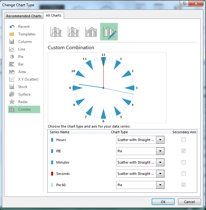
Building an Excel Clock Chart - Xcelanz
How to add axis label to chart in Excel? - ExtendOffice Add axis label to chart in Excel 2013. In Excel 2013, you should do as this: 1.Click to select the chart that you want to insert axis label. 2.Then click the Charts Elements button located the upper-right corner of the chart. In the expanded menu, check Axis Titles option, see screenshot:. 3.

Excel rotate radar chart - Stack Overflow
Excel charts: add title, customize chart axis, legend and ... Click the Chart Elements button, and select the Data Labels option. For example, this is how we can add labels to one of the data series in our Excel chart: For specific chart types, such as pie chart, you can also choose the labels location. For this, click the arrow next to Data Labels, and choose the option you want.
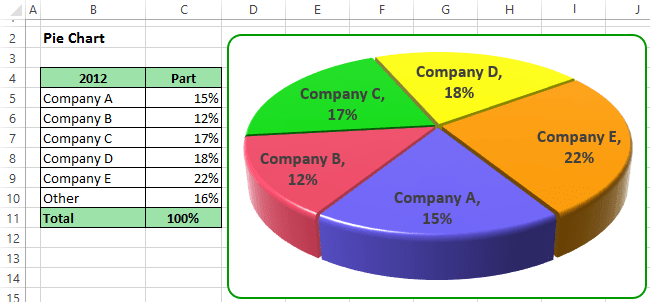
Excel 3-D Pie charts - Microsoft Excel 2013
Adding rich data labels to charts in Excel 2013 ... The data labels up to this point have used numbers and text for emphasis. Putting a data label into a shape can add another type of visual emphasis. To add a data label in a shape, select the data point of interest, then right-click it to pull up the context menu. Click Add Data Label, then click Add Data Callout. The result is that your data ...

Data labels on Excel charts « projectwoman.com
Adding 2nd Data Label Series to Bar of Pie Chart If you use 2 sets of the same data in the chart you can create 2 pie/bar charts, with one appearing on the secondary axis. Make sure the settings for bar/pie formatting are the same. Add data labels to each series. Format one to show names the other values. Within the pie you may want to delete the name data labels. Attached Files
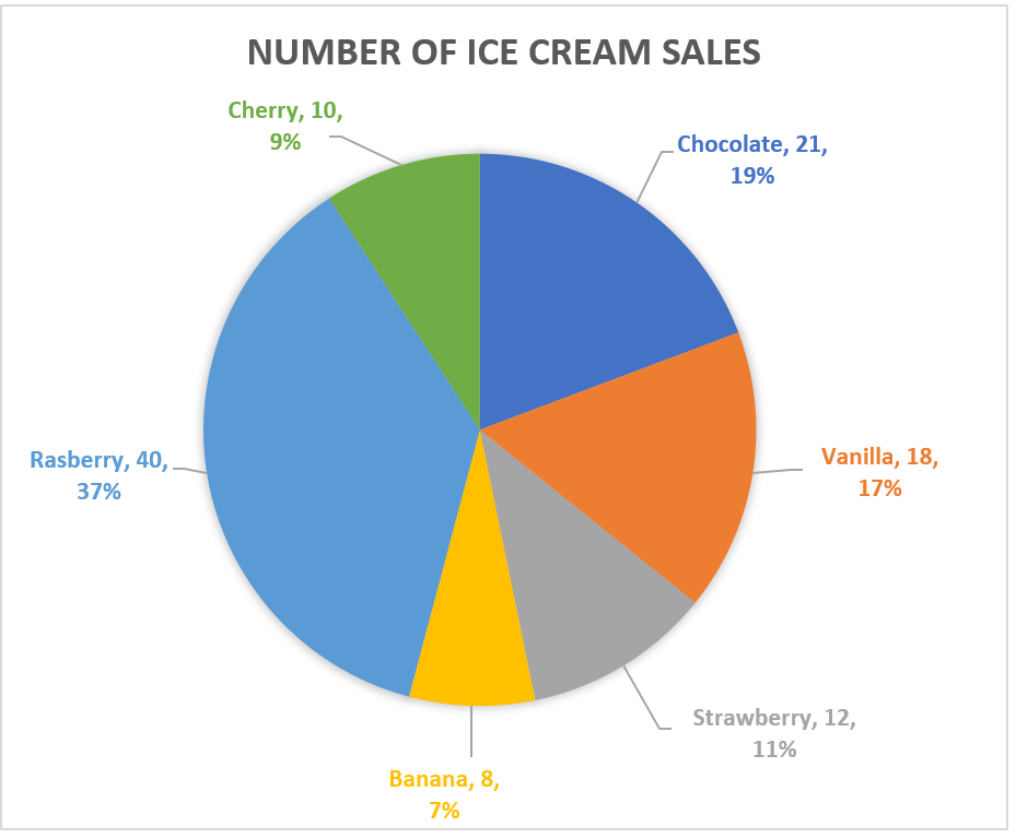
How-to Make a WSJ Excel Pie Chart with Labels Both Inside and Outside - Excel Dashboard Templates
How to Customize Your Excel Pivot Chart Data Labels - dummies To add data labels, just select the command that corresponds to the location you want. To remove the labels, select the None command. If you want to specify what Excel should use for the data label, choose the More Data Labels Options command from the Data Labels menu. Excel displays the Format Data Labels pane.

Do My Excel Blog: How to hide the zero percent labels in an Excel pie chart
How to Insert Axis Labels In An Excel Chart | Excelchat We will go to Chart Design and select Add Chart Element Figure 6 - Insert axis labels in Excel In the drop-down menu, we will click on Axis Titles, and subsequently, select Primary vertical Figure 7 - Edit vertical axis labels in Excel Now, we can enter the name we want for the primary vertical axis label.
10 Simple Steps on How to make a pie chart in Excel – Excel Wall
How to Create a Pie Chart in Excel | Smartsheet If want the category names to appear on or near the chart, right-click on the chart and click Add Data Labels …. By default, the numerical values are added. To add other labels, such as the categorical values or the percentage of the total that each category represents, right-click on the chart, then click Format Data Labels ….
Post a Comment for "44 excel pie chart add labels"